A Technical Note on the DoppelScout

Greetings friends,

A couple of weeks ago, we introduced DoppelScout with our first case on Mohamed Salah. Thanks again for all the feedback! Today’s drop is a bit different: it’s a deep dive into the technical side of DoppelScout. We're talking context layers, role modeling, system effects, basically, what powers the tool behind the scenes.

⚠️ Heads up: If you’re just here for game-day vibes and football stories, feel free to skip this one. No worries, your usual Dead Ball Digest will be back Monday as always. But if you're into the mechanics of modern scouting and love peeking under the hood, you're in the right place. Let’s dig in.

A Concise Overview of the DoppelScout

In our previous piece, we chose storytelling over equations, deliberately avoiding deep technical dives to make the DoppelScout's insights accessible and engaging. Nevertheless, behind the elegant visualisations and similarity scores lies a robust, evolving system grounded in data science and statistical theory. This report is for those curious minds who want to peek under the hood. We’ll walk you through the key components, logic, and structure behind the DoppelScout.

What is the DoppelScout?

The DoppelScout is a player similarity engine developed to identify players with stylistic and statistical proximity to a given target. It’s not just a similarity calculator, it integrates positional awareness, consistency over seasons, and adaptability to tactical roles.

Why Did We Build It This Way?

Player comparison isn’t linear. It’s not a clean equation of goals + assists or isolated brilliance. In modern scouting, you're dealing with a messy mix of contextual factors, roles, systems, data noise, and market madness. That’s why we needed the DoppelScout. Traditional scouting metrics (goals, assists, etc.) fail to capture the game’s complexity. DoppelScout treats player comparison like a recipe, mixing:

• Similarity metrics (statistical proximity)

• Role clustering (positional fit)

• Consistency checks (multi-season reliability)

• Graph‐based relationships

These elements combine into a weighted score, reflecting football’s “chaotic soup” of context and connections.

Case Study: Mohamed Salah

We deliberately chose a challenging benchmark to push the limits of the DoppelScout in its earliest version. Who better than Mohamed Salah, a player who defies simple categorisation? A right winger by position, a striker by numbers, a playmaker by instinct. Replacing the Egyptian King means replacing goals, assists, tactical intelligence, and positional fluidity. It’s the perfect stress test to expose the model’s strengths and areas for growth.

Core Data & Filtering

• Data Source: FBref’s Big 5 European Leagues (2017–18 to present)

• Features: 150+ metrics, normalised (per 90, per touch, share-of-team) for fair comparison

• Pre-filtering:

  • Age limits

  • Primary positions (from tactical data)

  • Minimum matches/minutes to ensure reliability

Acknowledged Limitations

• Feature Correlation: e.g., key passes vs. assists

• Data Gaps: Older seasons may be incomplete

• Coarse Roles: Only four broad categories (GK, D, M, F)

Rather than ignoring these issues, DoppelScout’s multi-stage pipeline compensates for them, blending raw comparisons with corrective layers.

Case Study: Mohamed Salah

We deliberately chose a challenging benchmark to push the limits of the DoppelScout in its earliest version. Who better than Mohamed Salah, a player who defies simple categorisation? A right winger by position, a striker by numbers, a playmaker by instinct. Replacing the Egyptian King means replacing goals, assists, tactical intelligence, and positional fluidity. It’s the perfect stress test to expose the model’s strengths and areas for growth.

Core Data & Filtering

• Data Source: FBref’s Big 5 European Leagues (2017–18 to present)

• Features: 150+ metrics, normalised (per 90, per touch, share-of-team) for fair comparison

• Pre-filtering:

  • Age limits

  • Primary positions (from tactical data)

  • Minimum matches/minutes to ensure reliability

Acknowledged Limitations

• Feature Correlation: e.g., key passes vs. assists

• Data Gaps: Older seasons may be incomplete

• Coarse Roles: Only four broad categories (GK, D, M, F)

Rather than ignoring these issues, DoppelScout’s multi-stage pipeline compensates for them, blending raw comparisons with corrective layers.

Figure 1: The DoppelScout Frameworks

Stage 1: Similarity & Distance

When comparing players, we’re essentially working with high-dimensional vectors:
Each vector represents a player’s statistical profile across ~150 normalised features (per 90, share-of-team, per shot, etc.). So, how do we measure the similarity between two such vectors?

There are many ways to define "closeness" in high-dimensional space. And no single metric is universally reliable. Here's why:

• Some metrics prioritise direction, not magnitude

• Some others emphasise absolute distance

• Some adapt to the underlying data structure

A Math Deep Dive? Come on! We previously said that distance IS NOT similarity: Let’s see this in a toy example, and say we model player performance as vectors in high-dimensional space (for simplicity, let’s work with three stats)

Let’s start with the Euclidean Distance (ED), which measures the raw difference in space: how far apart two players are, based on absolute numbers. It is expressed as

For Player B, it is

For Player C, it is

Now, let’s look at one of the most utilised similarity metrics among sports analytics scientists, the Cosine Similarity, which measures the angle between the vectors, focusing on pattern, not scale. Perfect for stylistic comparisons. It is expressed as

For Player B, it is:

For Player C, it is

Let’s return to the original question: Why do we use multiple similarity metrics? The toy example above makes it clear: No single metric captures the full picture. That’s why DoppelScout combines multiple (more than 5) similarity signals to strike a balance between: (i) Style vs. Production, (ii) Direction vs. Magnitude, and (iii) Normalised vs. Raw Performance. The scatter plot below illustrates why relying on a single similarity metric can be misleading, highlighting that only candidates with both high stylistic similarity (cosine) and low output difference (Euclidean) fall into the truly optimal region for DoppelScout.

Figure 2: High cosine alone ≠ good match (top-right). Low Euclidean alone ≠ good match (bottom-left). Only the bottom-right quadrant, where both metrics agree, yields reliable candidates.

Stage 2: Clustering & Dimensionality Reduction

While similarity metrics help us evaluate players individually, clustering allows us to understand how they group and relate to each other collectively. Clustering is the tool that lets us detect hidden structures in high-dimensional space without manually defining positional labels or player types. It helps DoppelScout answer questions like:

• “Is this player a lone outlier or part of a stylistic group?”

• “Are there clusters where our target is an outlier, and what does that imply?”

• “Which players are statistically and stylistically grouped with our target?”

Clustering adds a layer of context on top of similarity. Instead of just “who is similar,” we ask, “What type of player is this, and who else belongs to that type?” Moreover, it allows us to filter out false positives: players who may be similar in stats but belong to a different stylistic group. And it also supports role awareness without needing rigid position labels. The most common types of clustering algorithms are K-Means (geometry-based), H/DBSCAN (density-based), Hierarchical, and many others.

At its core, clustering algorithms group vectors in a way that maximises within-cluster similarity AND minimises between-cluster similarity. So, let’s assume we have a dataset

where we have n players, each of which refers to a d-dimensional vector (belonging to d different statistics). We aim to partition this dataset into K clusters

such that

This means that merging all clusters boils down to the dataset X, and none of the players are in the same cluster.

Assume D(⋅) is a dissimilarity function; regardless of the algorithms, any clustering method tries to minimise player dissimilarity within a group (intra-cluster) whilst trying to maximise dissimilarity between groups of players (inter-cluster). Mathematically speaking:

Figure 3: The Theory of Clustering Algorithms

Different algorithms utilise different dissimilarity functions, such as:

• K-Means: Uses squared Euclidean distance to centroids

• DBSCAN: Uses density and neighbourhood connectivity

• Hierarchical: Uses linkage distances between merged groups

As a summary, Clustering is the task of learning a function😀 

which assigns each data point (player) to a cluster, where the function respects the similarity structure inherent in the data.

We embed clustering within the DoppelScout pipeline not just as a technical layer, but as a lens into the footballing ecosystem around the target player. It enables us to:

• Understand which stylistic group a player belongs to

• Avoid comparisons across irrelevant roles or tactical archetypes

• Treat similarity differently depending on the group context

This means a winger isn’t flagged just because their numbers (e.g. high xG) resemble a striker’s unless their underlying behavioural cluster justifies the overlap (Wingers like Salah, Yamal, and Vini Jr, who also take a role as centre forwards). After clustering, we operate in a refined space that gives us more than just raw proximity, it gives us contextual distance. That’s all we’ll say for now.

Call it a soft guardrail: similarity alone might suggest a match, but clustering helps us ask, “Do they belong in the same footballing neighbourhood?”

Choosing the Number of Clusters: Determining how many clusters to form is a fundamental challenge in unsupervised learning. Since clustering is not guided by labelled outcomes, we rely on model selection criteria to evaluate the quality of different groupings. Common techniques include the Elbow Method, where we look for diminishing returns in variance reduction; Silhouette Analysis, which assesses how well each point fits within its assigned cluster; and Gap Statistics, which compares observed clustering against random baselines. The goal isn’t to find a “perfect” number but to find a stable, interpretable structure that reveals genuine player archetypes without overfitting.

Why Dimensionality Reduction Comes First: Before clustering, we apply dimensionality reduction to simplify the complex, high-dimensional player vectors. With over a hundred statistical features per player, the raw space can be noisy, redundant, and hard to separate meaningfully. Dimensionality reduction techniques like Principal Component Analysis (PCA), UMAP, or t-SNE help project this data into a lower-dimensional space where the underlying structure is clearer, and distances become more meaningful. This step not only improves clustering quality but also allows for visual interpretation, enabling us to see how stylistic clusters form concerning each other and the target player.

Stage 3: Consistency & Uncertainty

• “Did this player shine only for a single season or maintain his performance year after year?”

• “How much can we trust the stats; are they stable, or could they swing wildly next season?”

Football performance isn’t static. A player might explode onto the scene with a standout year, only to regress or plateau later. In scouting, distinguishing a genuine trend from a one-season wonder is crucial. This is why the DoppelScout’s evolution considers longitudinal analysis – looking at a player’s output over multiple seasons. We want to gauge consistency: is the player reliably excellent or riding a temporary high? Likewise, we assess uncertainty: how much statistical volatility is in their profile. A player with 15 goals one season and 3 the next presents a different risk profile than one who scores 8-10 every year. High variance might signal inconsistency (or changing roles, injuries, etc.), which impacts how a scout interprets the similarity.

Mathematically, consistency can be viewed through variance and sample size. Intuitively, the larger and steadier a player’s body of work, the more confidence we have in their “true” level. For example, we trust that rate if Player X averages 0.4 goals/90 minutes with a small standard deviation over five seasons. If Player Y averages 0.4 as well but with huge swings (0.8 one year, 0.0 the next), we attach more uncertainty to his profile.

On the other hand, variance alone might sometimes be problematic when used to measure consistency. While variance captures the overall spread of values, it is highly sensitive to outliers and disproportionately influenced by extreme observations. To illustrate this nuance, we examine the scoring output (goals per 90 minutes) of six forwards who have played across the Big 5 European leagues over the past seven seasons.

Figure 4: Distribution of Goals per 90 Minutes Between 2017–18 and 2023–24 Across Six Forwards, with annotated interquartile range and standard deviation.

Each player’s boxplot shows the distribution of seasonal G/90 values, with annotated variance and interquartile range (IQR) — the middle 50% of their data. While variance gives a broad sense of volatility, IQR offers a more robust measure of scoring stability, particularly when outliers are present.

• Mo Salah, Olivier Giroud, and Erling Haaland are classic examples of consistent performers, with both low variance and tight IQRs (~0.09–0.10). Notably, Haaland’s low variance is particularly impressive given his high goal output.

• Lukaku displays a slightly wider IQR and low variance, placing him in the moderate consistency tier.

• Timo Werner and Ousmane Dembele, meanwhile, have higher variances (0.045 and 0.073, respectively), but it is the IQR values (0.20 and 0.36) that truly highlight their inconsistent scoring patterns, even beyond what variance alone suggests.

This visual comparison reinforces why IQR can be a more stable and interpretable indicator of consistency in scouting contexts. While both metrics are informative, IQR avoids being skewed by statistical outliers and better reflects the "normal" range of performance a scout or analyst can expect from a player season over season. In a DoppelScout context, volatile players might be de-emphasised or flagged, since a high similarity score based on an outlier season could mislead. We prefer those who consistently exhibit the target’s traits, rather than a player who only occasionally hits those heights.

The rationale is simple: scouting decisions live in the future, so we must account for how reliably a player’s past performance predicts future output. By incorporating consistency and uncertainty measures, DoppelScout will better distinguish a reliable match from a risky mirage. This addition will make the engine more robust, tempering pure similarity with a measure of confidence in that similarity. In short, the model will learn to ask not just “How similar is this player to our target?” but also “How sure are we of that similarity?”.

Stage 4: Graph Theory

• “How does our target connect to others in the web of playing styles?”

• “Is he a unique island, or one of many similar players? And who are the bridges linking different styles?”

When we talk about similarity, it’s natural to envision a network. Imagine each player as a node in a graph, with edges linking players who play alike. The stronger the similarity, the thicker or shorter the edge. Instead of looking at players in isolation, DoppelScout can examine this player similarity graph to uncover deeper insights. Graph theory gives us tools to quantify a player’s role in this stylistic web. Are they central within a cluster of similar players, or on the periphery? Do they connect multiple clusters? This perspective is especially useful for understanding contextual importance – it’s one thing to find a player similar to our target, but another to understand how that player sits in the broader ecosystem of football styles.

In our graph model, each node is a player, and each weighted edge reflects the degree of stylistic similarity between two players. To enrich our understanding, we use several network measures. Eigenvector centrality acts like a "popularity score"; it favours players connected to others who are themselves well-connected. A high eigenvector score means a player is a prototypical figure within their style cluster, while a low score might flag a niche or unconventional profile. Betweenness centrality, on the other hand, highlights players who act as bridges between different clusters; stylistic hybrids who link otherwise distant archetypes. These may not be central within a group but are strategically placed in the network, often making them tactically flexible or system adaptable.

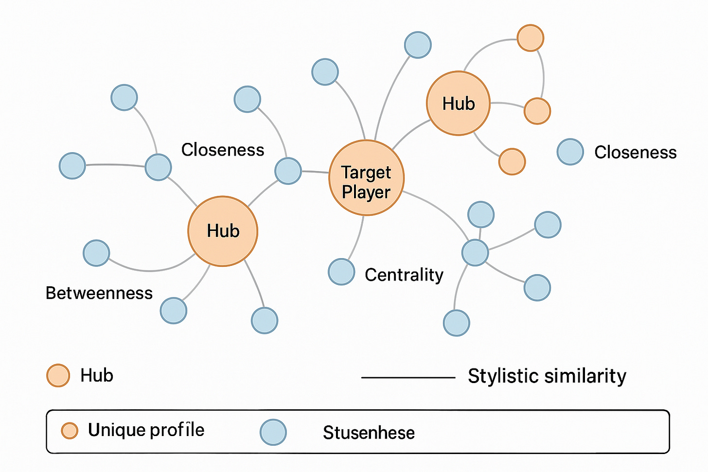
Figure 5: A conceptual player similarity network where nodes represent players and edges reflect stylistic similarity. The target player is highlighted. Graph-based metrics like eigenvector centrality, closeness, betweenness, and local density help evaluate a player’s role within the stylistic ecosystem, identifying whether they are hubs, bridges, or outliers in their footballing archetype.

Closeness centrality measures how quickly a player can “reach” others, in stylistic terms, how many small adjustments it would take to resemble them? A high closeness score suggests a versatile and broadly relatable style; a low score often means a player is stylistically isolated. We also consider local density, which reflects how tightly knit a player’s immediate neighbours are. A player embedded in a dense cluster is surrounded by many lookalikes, implying replaceability. However, a player in a sparse region might possess a more unique blend of traits. By combining these metrics, we move beyond binary similarity and start asking more nuanced questions: Is this player central or fringe? Typical or rare? A bridge or an island? That context shapes how we interpret similarity and influences the final DoppelScore.

Let’s do some maths again; formally, we represent the player similarity space as a weighted, undirected graph

where

From this graph, several centrality measures are derived:

Eigenvector centrality solves

where A is the adjacency matrix of G, and x gives influence scores for each node based on connectedness to other influential nodes.

Closeness centrality for a node v is defined as

where d(v,u) is the shortest path distance, intuitively, how “far” the player is from others.

Betweenness centrality quantifies how often a node appears on the shortest paths between all other pairs:

where

Let’s also see them in a figure:

Figure 6: Visual illustration of four key graph centrality metrics, each of which captures a different structural role: eigenvector centrality highlights influence through well-connected peers, closeness captures global proximity, betweenness identifies bridges between clusters, and local density reflects how tightly connected a player’s immediate neighbourhood is.

Each of these metrics contributes a different perspective on how players are situated within the broader stylistic network, allowing DoppelScout to identify not only how similar players are to the target but also how important or replaceable they are in the context of football’s tactical map.

We don’t explicitly reveal how these graph metrics feed into the secret sauce, but the logic is straightforward: network context refines similarity. Graph theory adds a layer of understanding about rarity and prototypicality if a candidate is statistically similar to the target (Stage 1) and in the right cluster (Stage 2). For instance, an option might be very similar to our target but also akin to dozens of other players (high eigenvector, high closeness), perhaps indicating his skills are more replaceable or come in an environment that flatters many players. Another option might be similarly close to the target but an outlier in the network (low centralities); a unique gem who, if truly matching the target, could be a special like-for-like replacement but with a smaller margin for error (since few comparables exist). By modelling the game as a graph of similarities, DoppelScout ensures we account for these subtleties. It helps answer questions like, “Is our target in a dense neighbourhood of similar players, or is he out on a stylistic limb?” and “Where does a given candidate lie, a centrepiece of a style cluster or an odd fit who happens to overlap with our target?” These insights guide how we weigh and interpret the final recommendations.

Stage 5: DoppelScore Calculation – Fusing the Ingredients

• “Can we distil all this complexity into a single score without losing the plot?”

• “How do similarity, role fit, consistency, and network value come together to rank our targets?”

This stage is the grand finale in terms of the magic of Data Science and AI; the moment where all components are combined into one actionable index: the DoppelScore.

Up to now, we’ve gathered a wealth of signals about each candidate: how closely they mirror the target’s stats and style (Stage 1), whether they belong to the same tactical family (Stage 2), how steady and reliable their outputs are over time (Stage 3), and what the similarity network says about their profile’s prominence or uniqueness (Stage 4). The DoppelScore is where we blend all these ingredients into a single number that allows easy comparison of candidates. Importantly, this score is not a trivial average; it’s a weighted composite crafted to reflect what we (and scouts) value most in finding a replacement. (The exact recipe remains proprietary, but conceptually, each component influences the final score in proportion to its importance for the role in question.)

Think of the DoppelScore as a similarity-and-fit index. A high DoppelScore means the candidate checks most of the boxes: stylistic match, role suitability, consistent performance, reasonable network context, and complementary traits like versatility. A lower score indicates some mismatch or concern in one or more areas. Let’s break down the key components that feed into the score:

• Statistical Similarity: This is the core comparison of the player’s stats/profile to the target’s. It encompasses multiple metrics (as discussed in Stage 1) to ensure we capture style (e.g. how a player achieves their numbers) as well as volume. A strong match here means the player “plays” like the target in measurable ways.

• Cluster Fit: Drawing from Stage 2, this reflects whether the player comes from the same stylistic cluster or role grouping as the target. If our target is an attacking midfielder/wing hybrid, a candidate from that same cluster gets a boost versus someone who might have similar stats but belongs to a different archetype. Cluster fit ensures we respect context – it’s a proxy for tactical role equivalence.

• Consistency & Uncertainty: When active, this factor will adjust the score based on the reliability of the player’s performance. A candidate who has delivered 3+ seasons of target-like performance will be rated higher than one who only flashed that level briefly. We essentially plan to penalise volatility; high uncertainty will drag a score down a bit, reflecting the added risk. (In v1, this is mostly handled by our filtering and by scouts’ interpretation, but in v2, the score itself will likely incorporate a consistency coefficient.)

• Graph Network Metrics: We incorporate insights from Stage 4 in subtle ways. For example, a candidate whose style is extremely rare might actually get a small lift if that matches an equally rare target (because that uniqueness is exactly what we need). Conversely, if a candidate is similar but lives on the fringe of the network in a different cluster, that might temper the score. Additionally, being a well-connected “hub” player (high eigenvector centrality in the similarity graph) could be seen as a positive – it often means the player excels in a style that is proven and recognised (many comparable peers). These graph-based adjustments are nuanced, ensuring that we don’t purely look at the candidate in a vacuum but also in the landscape of available talent.

After weighing and mixing these factors, the DoppelScore emerges as a single figure. What does this number mean to a user? In essence, it’s our model’s holistic verdict on “How close is Player X to being a doppelgänger of the target in overall profile and fit?” A score of, say, 90+ would indicate a very strong match on most fronts; something around 60 might indicate a partial match or a player who mimics many aspects but perhaps falls short in one area (or carries more uncertainty). We generally don’t expect a perfect 100 (even 90s); after all, even the most similar player will have differences, but the score allows easy ranking of candidates from most to least alike. It’s important to stress that a higher DoppelScore isn’t necessarily a prediction of success (football isn’t that simple!), but it’s a signal that the player warrants serious consideration as a successor or alternative to the target.

At its core, the DoppelScore is calculated as a weighted sum of multiple components, each reflecting a different layer of similarity or fit:

where:

Each term is normalised between 0 and 100, ensuring the final DoppelScore remains interpretable on a 0–100 scale. This formulation allows us to capture both closeness and context, not just how similar a player is, but also how relevant and reliable that similarity is.

One of the core strengths of this approach is its adaptability. By adjusting the weights w, scouting teams can prioritise what matters most in their context:

• Emphasising S yields direct stylistic matches; good for plug-and-play replacements.

• Emphasising C helps focus on role equivalence; valuable when system fit is non-negotiable.

• Weighting G more can highlight network archetypes or identify rare profiles.

• And tuning U ensures reliability, especially when projecting long-term success.

This flexibility ensures that DoppelScout isn't a one-size-fits-all tool. It becomes a customizable engine that reflects each club's recruitment philosophy, tactical identity, and risk appetite.

To make the above explanations concrete, let’s use an example from our first results. Consider our case study target, Mohamed Salah, and one of the candidates (actually 1^st with the highest DoppelScore), the DoppelScout highlighted: Omar Marmoush (a young Egyptian forward). How might Marmoush’s profile translate into these components and ultimately his DoppelScore?

• Similarity: Marmoush’s statistical profile shows a Salah-like inclination to dribble and cut inside to shoot. His cosine similarity to Salah’s recent-season vector is high – for instance, he has a similar ratio of shots, touches in the box, and take-ons. On raw production, of course, he’s lower (Salah plays for Liverpool; Marmoush was at Frankfurt with fewer goal contributions), but after normalising for team context, he still registers as a smaller-scale Salah in style. This gives him a strong base similarity score.

• Cluster: The clustering analysis places Marmoush in the inside forward/winger cluster, the same general family as Salah. He’s not miscast; we’re not comparing Salah to a pure striker or a midfielder here. Marmoush’s peers in his cluster are the likes of mobile-wide forwards; exactly the sandbox we’d want to be in to find “the next Salah.” This cluster alignment reinforces his candidacy (no red flags of a role mismatch).

• Consistency: Here is an area of slight caveat: Marmoush is a younger player with fewer seasons at the top level. The data we have from him (mostly two seasons of regular play) show a fairly steady output – he didn’t have wild swings, but the sample is limited. Salah, by contrast, has been elite for many seasons running. In a future version, the model might down-weight Marmoush’s score a bit for lack of long-term proof. In v1, it’s noted qualitatively that scouts would recognise the smaller track record. Still, nothing in Marmoush’s history screams inconsistency – he just hasn’t had the scope to prove longevity yet.

• Graph Metrics: On the similarity network, Marmoush is connected to Salah (by design, since he was found as similar) and also links to other winger-forwards. However, Salah’s eigenvector centrality in the network of attackers is very high (he’s similar to many notable players and essentially defines a style), whereas Marmoush’s is modest – he’s connected to a subset of players and is a bit more peripherally placed in that network (partly because he’s still making his mark, and partly because his performance level is just a tier below top class). Marmoush’s closeness is reasonably high; he’s not an oddball outlier – he’s just not a central hub. In practical terms, this tells us Salah is a proven template for success (hence many players try to emulate aspects of his game), while Marmoush is a promising prospect who ticks similar boxes but hasn’t become a hub player in the network. The DoppelScore algorithm interprets this as: Marmoush is stylistically on point but perhaps not as “guaranteed” a hit, which aligns with common sense.

  

Figure 7: Mo Salah and Omar Marmoush – 2024-25 Big 5 League Last 365 Day Statistics and percentiles.

Now, when the model fuses these aspects, Marmoush ends up with a strong DoppelScore (let’s say hypothetically in the high 70s out of 100). That score encapsulates “Marmoush is quite similar to Salah in style and role, with some questions about proven consistency and overall impact (as expected for a younger player).” A scout reading this would understand that Marmoush is one of the closest matches to Salah’s profile available, and the areas where he differs (experience, current output volume) are exactly where you’d do further due diligence. This is precisely the goal of the DoppelScore – not to declare someone “Salah 2.0” with absolute certainty, but to provide a concise summary of multi-faceted similarity. It’s a final heuristic that brings all the model’s learnings together, making the complex comparison of dozens of players digestible. The top-ranked names by DoppelScore become our shortlist. And as we’ll see next, that short list isn’t the end of the story – it’s the start of human exploration.

Stage 6: Human-in-the-Loop Filtering

Even the best DoppelScore needs a final reality check; this is where scouts, analysts, and decision-makers add context that data alone can’t capture. After the model ranks candidates, humans filter them through six practical lenses:

• Transfer Feasibility: Is the player actually for sale (contract length, rival club, release clause)?

• Health & Durability: Does their injury history undermine their availability?

• Character & Mentality: Will they fit the dressing room and maintain professionalism?

• Tactical Nuance: Do they press, track back, or satisfy specific system demands?

• Age & Development: Does their career stage match the club’s strategic timeline?

• Cost vs. Value: Which option offers the best style–price balance?

By combining quantitative rigour with this qualitative vetting, DoppelScout hands over a shortlist that’s both statistically sound and practically viable.

Figure 8: A modern scouting workflow, where data-driven insights and expert intuition come together to finalise the shortlist.

Limitations & Open Challenges

No model is perfect, and the DoppelScout is no exception. While we’re proud of the system’s early results, it’s important to be clear about its current limitations and the open challenges we face moving forward. Transparency about these aspects ensures that users understand the tool’s boundaries and helps guide future development. Here are some key limitations and challenges:

• Data Constraints: We rely on public, aggregate Big-5 European Leagues’ stats (no tracking, off-ball events or global coverage), so we miss fine-grained movement and context signals.

• Role Granularity: Broad position buckets (“Forward,” “Midfielder,” etc.) and clustering can’t perfectly capture rare or hybrid roles, leading to occasional misclassifications.

• Model Simplification: Reducing a player to a vector score overlooks leadership, adaptability, and team context; factors that demand human interpretation.

• Limited Understanding of Causality: Similar stats don’t guarantee similar playing styles or motives; our human-in-the-loop filters help flag false positives.

• Dynamic vs Static Performance: Using historical data means we can’t forecast a player’s development curve, so rising talents or fading veterans may be misranked.

• User Interpretation and Trust: As a “black box,” DoppelScout needs explainable outputs and interactive tools to build confidence and clarity.

Despite these challenges, the foundation is in place, and future data partnerships, refined role definitions, and dynamic modelling will help us close these gaps.

Figure 9: Behind every algorithm lies a set of assumptions, and in this room, we’re actively challenging them.

Future Steps

DoppelScout v1 is just the beginning. We're building a platform that continuously evolves; more nuanced, more scalable, more global. Here’s what’s next:

• Event Data Integration: We’re moving from what happened to how. By incorporating granular event data, pass types, directions, locations, and context, we’ll give the model “eyes” on player decision-making. This includes touch maps, build-up involvement, and stylistic tendencies like overlapping vs. underlapping. It’s a technical leap, but it’s coming soon.

• Tracking Data (Long-Term): Beyond events, tracking data offers the holy grail: off-ball movement, pressing intensity, space occupation. This will allow DoppelScout to understand how a player behaves without the ball, something currently only a human scout can see. It’s complex and heavy, but we believe this will define scouting 3.0.

• Global League Expansion: Currently focused on the Big 5 leagues, we aim to expand to the Netherlands, Portugal, Brazil, Argentina, MLS, and beyond. This isn’t just for scale; it’s about finding under-the-radar talent that mimics elite profiles. With proper normalisation, DoppelScout will help spot “the Salah of South America” or “a Mahrez in Eredivisie.”

• Real-Time Updates & Alerts: We’re working toward a living system, one that refreshes weekly or even daily. Soon, the tool could alert scouts to emerging matches in real time: “Over the last 5 games, Player X has developed a profile very close to Salah.” That’s proactive scouting.

• Interactive Explorer: We’re currently conducting our feasibility study of building a visual Explorer interface where users can filter, adjust weighting, explore the player network, and compare candidates directly. It transforms DoppelScout from a black-box engine into a sandbox, letting scouts ask, “What if?” (counterfactual reasoning) and get dynamic, data-backed answers.

• Feedback Loops: Eventually, the system will learn from scouts. If suggestions are consistently ignored or praised, we’ll build semi-supervised learning to refine how the model understands “good fit.” The goal: an adaptive tool that learns from the field, not just the data.

Figure 10: A young dreamer imagines a world where data can unlock talent from every corner of the globe.

Closing Thoughts

DoppelScout began with a question: Can we find the next Salah, and prove it with data? That challenge sparked a modular system that combines similarity, clustering, consistency, network theory, and human feedback. Every stage can evolve independently, keeping the whole system agile.

This isn’t a tool built to replace scouts; it’s built to enhance them. A scout used to start with a hunch. Now, the data can start the conversation. It’s a partnership, human intuition and data intelligence working together.

Figure 11: A Chief Scout celebrates a breakthrough suggestion delivered not by chance, but by a trusted AI assistant.

We’ve built something relatively powerful with just open-access data. No tracking, no proprietary event feeds, yet we're already surfacing players that match tactical fingerprints. Imagine what DeadBall Analytics could do with deeper data, broader reach, or strategic backing. If you’re a data provider, investor, or strategic partner reading this — yes, you — imagine what we could accomplish together.

The journey has just begun. Version 2 will be smarter. Version 3 will be faster. Football is chaotic and magical; our job is to make sense of it, not simplify it. DoppelScout won't eliminate the mystery, but it can reveal the patterns. It’s scouting with a new lens; one that looks forward, learns continuously, and never stops evolving.